Quickstart Guide
Welcome to the quickstart guide for DART!
DART is a python package to generate approximate 3D structures of transition metal complexes from a large database of 41,018 distinct ligands, the MetaLig ligand database. The ligands were curated from more than 100,000 transition metal complexes from the Cambridge Structural Database (CSD) and cover a wide chemical space with denticities ranging from monodentate to decadentate ligands, and even including haptically coordinating ligands.
DART is like LEGO for transition metal complexes: the building blocks are atoms (for the metal centers) and ligands from the MetaLig. Users specify the chemical space (geometry, metal centers, type of ligand) they want to explore, and DART will automatically query the MetaLig database for all ligands that fit the criteria, assemble all possible combinations of ligands (or a random subset), and save the generated complexes as .xyz and .json files. The generated structures are approximate, but they are a great starting point for further geometry optimizations with quantum chemistry methods such as DFT.
As an introductory example, we will walk through the process of assembling 100 square-planar neutral Pd(II) complexes. Each complex will feature one cis-bidentate ligand and two monodentate ligands. We will first assemble complexes using randomly sampled ligands from the MetaLig, without targeting any particular chemical space. Then, we will learn how to filter down the input ligands in order to generate complexes targeted to a certain chemical space and to generate those that are more likely to form stable complexes.
Confirm DART Installation
This tutorial assumes that you have already installed DART by following the instructions in the installation guide. Before starting, ensure DART is correctly installed and configured:
Open your terminal.
Type
DARTassembler --helpand press Enter.
This command should display a help message listing all available DART modules. If you encounter any errors, please refer to the Troubleshooting and FAQs section for assistance.
Code along and visualize the results with ase
We invite you to code along with this tutorial. Reading is good, but doing is better! DART is a command-line tool, so you will need to use your terminal to run the commands. Each section provides code snippets that you can copy-paste into your terminal.
DART relies on the excellent ase (Atomic Simulation Environment) package, which is installed automatically along DART. Additionally to its use in the python code, we will also use the ase gui terminal command in this tutorial to visualize 3D atomic structures saved as .xyz files, such as the ligands in the MetaLig database or the generated complexes. The syntax to visualize a .xyz file with ase is always ase gui FILENAME.xyz.
Make a Working Directory for this Tutorial
Let’s start by creating a new directory for this tutorial and navigating into it:
mkdir DART_quickstart
cd DART_quickstart
Explore the Ligand Database
To explore the MetaLig ligand database, use the dbinfo module:
DARTassembler dbinfo --db metalig --n 5000
You can read this command as follows: use the dbinfo module of DARTassembler, and for this module specify the options --db metalig as a shortcut to the full MetaLig database, and --n 5000 to only load the first 5,000 ligands from the database to speed up this example. You can of course load the entire database by omitting the --n option, but for this quickstart tutorial we want to keep things fast. Later, you can also read in custom ligand database files by providing the path to the file instead of --db metalig, e.g. --db /path/to/your/ligand_db.jsonlines.
The above command will immediately save two files. The first file is a concatenated .xyz file with the 3D structures of all the ligands. You can visualize and browse through the structures of the ligands by typing ase gui concat_MetaLigDB_v1.1.0.xyz in your terminal. The gui will open with three tabs. The left one shows the 3D structure of the ligand, the middle tab you can ignore, and in the right tab you can scroll or play a slideshow to browse through the ligands. You can also drag each tab out of the main window to create a new window, so you can view the 3D structure and the option for scrolling at the same time. The structures will show you a wide variety of ligands. Each ligand is coordinated to a dummy Cu metal center for visualization purposes only; the actual ligand is without the Cu atom. The Cu atom is placed at the location of the original metal center from the CSD entry from which this ligand was extracted, which also coincides with how the new metal centers will be placed when assembling new complexes with DART in the assembler module.
The other file saved is a .csv file called MetaLigDB_v1.1.0.csv. You can open this file with any program that can read .csv files, such as Excel or LibreOffice Calc, and view the ligands properties such as stoichiometry, denticity, donor atoms, charge, etc. Feel free to explore the database and get a feel for the ligands available in MetaLig!
Assemble Novel Complexes
To use the Assembler Module, we need to provide an input file which outlines all settings for the assembly. Please create a new file called assembler.yml and copy-paste the settings below. All the options are briefly explained as comments in the file:
# file: assembler.yml
output_directory: 'DARTassembler'     # Output directory for saving all results
n_max_ligands: 5000           # Max number of ligands to load from the database
batches:
  - name: 'PdII'              # User-defined name
    metal_centers: 'Pd'       # Metal center
    total_ligand_charges: -2  # Total charge from all ligands, to define neutral Pd(II) complexes
    ligand_db_files: 'metalig'  # Path to ligand database file or `metalig` for full MetaLig
    ligand_archetypes:
        - '2-cis'             # Bidentate ligand
        - '1-mono'            # Monodentate ligand 1
        - '1-mono'            # Monodentate ligand 2
    target_vectors:
        - ['+x', '+y']        # Bidentate ligand along +X and +Y axes
        - ['-x']              # Monodentate ligand 1 along -X axis
        - ['-y']              # Monodentate ligand 2 along -Y axis
    n_max_complexes: 100      # Number of complexes to generate
The options are as follows: we want to generate neutral Pd(II) complexes, so we set the metal_centers to Pd and the total_ligand_charges to -2, such that the -2 charge from all ligands balances the +2 charge from the Pd(II) center to give neutral complexes. We want to use the entire MetaLig database, but only load the first 5,000 ligands to speed up this example, so we set ligand_db_files to metalig and n_max_ligands to 5000. We also set n_max_complexes to 100 to only generate 100 random complexes (but all isomers of each complex).
The ligand_archetypes and target_vectors have a 1:1 relationship: they specify options for each binding site, so they must have the same number of entries, and they are read in the same order. The ligand_archetypes specify the type of ligand to assemble, here one cis-bidentate ligand (2-cis) and two monodentate ligands (1-mono, 1-mono). The ligands are then arranged around the metal center according to the target_vectors, where the metal center per default occupies the origin of the Cartesian coordinate system (0, 0, 0), and the location of each ligand is defined by a vector in Cartesian coordinates. For example, '+x' is short for the the Cartesian vector (1, 0, 0). The target_vectors in the above file thus define a square-planar geometry for the Pd(II) complexes, as shown in Figure 1 below:
['+x', '+y']: the first ligand (the cis-bidentate) will be coordinated to the metal center along the +X, +Y axes. The list has two entries because the2-cisligand has two donor atoms. Instead of the abbreviation['+x', '+y'], you would get identical results by providing the full Cartesian vectors[[1, 0, 0], [0, 1, 0]].
['-x']: the second ligand (monodentate) will be coordinated along the -X axis. The list has one entry because the1-monoligand has one donor atom. Instead of the abbreviation['-x'], you would get identical results by providing the full Cartesian vector[[-1, 0, 0]].
['-y']: the third ligand (monodentate) will be coordinated along the -Y axis. The list has one entry because the1-monoligand has one donor atom. Instead of the abbreviation['-y'], you would get identical results by providing the full Cartesian vector[[0, -1, 0]].
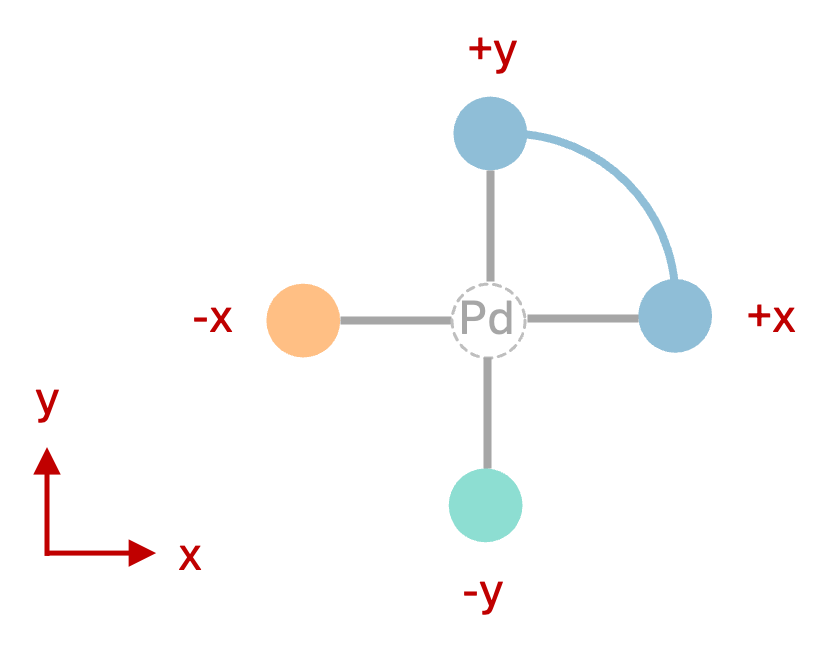
Figure 1: Square-planar complex geometry defined by the target_vectors above. The unconnected green and orange balls represent the two monodentate ligands, the connected blue balls represent the cis-bidentate ligand.
This was a small example, but DART supports the assembly of arbitrarily systems from 22 different ligand coordination archetypes. For more information on how to assemble more complex systems such as tetrahedral or octahedral complexes, please refer to the assembler module documentation.
Now execute the following command in your terminal:
DARTassembler assembler --input assembler.yml
The assembler module prints the progress to the terminal and saves the output files in the DARTassembler folder. You can get an overview of the assembled complexes by opening the file isomers.csv with a program such as Excel. This file displays information on all isomers of all complexes DART tried to assemble. DART automatically generates all possible geometric isomers, which is why most of our Pd(II) complexes in the csv file have 2 successful entries. However, you will notice that some complexes have only one or even zero successful isomers, which indicates they were filtered out due to steric clashes or duplicates (e.g. if the chosen cis-bidentate ligand is symmetrical). In total, we see 186 isomers of 100 complexes were successfully assembled, meaning most complexes have two valid isomers generated.
Now, we can also browse through all successfully assembled structures by opening the concatenated .xyz file with the ase gui:
ase gui DARTassembler/batches/PdII/concat_passed_isomers.xyz
Browsing through the assembled structures, you will notice that using the entire MetaLig database without any filters results in a very diverse chemical space. In the following section, we will learn how to filter the ligands to generate complexes with more chemically uniform structures.
Feel free now to play with the target vectors and see what happens when you provide other sets of target vectors. Can you swap the cis/trans orientation of the two monodentates relative to the bidentate? For more information on these settings, and especially the target vectors, please refer to the assembler module documentation.
Please close the ase gui window now before proceeding to the next section.
Target Chemical Space
You can achieve a more targeted exploration of TMC chemical space by employing the LigandFilters Module. This module allows you to filter the MetaLig by providing an input file with configurations for each pre-implemented filter. For example, let’s suppose we want to generate Pd(II) complexes with
one Br
one haptic C-donor with exactly 6 haptic donors
one N-N cis-bidentate ligand with at least one carbonyl group and history of coordinating to Pd, Pt or Ni in the CSD
The last option can be very useful to increase the likelihood that our Pd complexes will be chemically viable, since the ligands have precedent coordinating to a metal center from the same group.
We will now use the LigandFilters Module to filter the MetaLig database down to ligands that meet these criteria. Please create one configuration file for each ligand site, named Br.yml, haptic.yml and N-N.yml, and copy-paste the following settings into each file:
# file: Br.yml
outpath: 'Br.jsonlines'
n: 5000
filters:
  - filter: 'composition'
    elements: 'Br'
    instruction: 'must_contain_and_only_contain'
    only_donors: False
# file: haptic.yml
outpath: 'haptic.jsonlines'
n: 5000
filters:
  - filter: 'property'
    name: 'archetype'
    values: ['1-mono']

  - filter: 'composition'
    elements: 'C6'
    instruction: 'must_contain_and_only_contain'
    only_donors: True
# file: N-N.yml
outpath: 'N-N.jsonlines'
n: 5000
filters:
  - filter: 'property'
    name: 'archetype'
    values: ['2-cis']

  - filter: 'composition'
    elements: 'N'
    instruction: 'must_only_contain_in_any_amount'
    only_donors: True

  - filter: 'smarts'
    smarts: '[C](=[O])'
    should_contain: True

  - filter: 'parents'
    metal_centers: ['Pt', 'Pd', 'Ni']
Now, run the LigandFilters module:
DARTassembler ligandfilters --input Br.yml
DARTassembler ligandfilters --input haptic.yml
DARTassembler ligandfilters --input N-N.yml
The Br filter returns just 1 ligand, the haptic C-donor filter returns 42 ligands and the N-N cis-bidentate filter returns 24 ligands, making 1,008 possible complexes. If we would have used the entire MetaLig database instead of the small test set of 5,000 ligands, the numbers would be much higher: 294 haptic C-donors and 215 N-N cis-bidentate ligands, enabling the generation of 63,210 distinct complexes or 126,420 isomers!
Each filter process creates a new ligand database file (e.g. N-N.jsonlines) containing only the ligands that passed the filter criteria. Additionally, a new directory called info_N-N is created, containing detailed information about the filtering process. You can use this information to verify that the filters worked as intended. For example, let’s check that all the N-N bidentate ligands contain at least one carbonyl group by visualizing all ligands that passed the filter:
ase gui info_N-N/concat_xyz/concat_Passed.xyz
After inspection, please close the ase gui window before proceeding to the next section.
Assembling Complexes with Targeted Chemical Space:
Now, we will redo the assembly process with the refined ligand database. First, we update the assembler.yml file by appending a new batch that uses the filtered ligand databases:
# file: assembler.yml
output_directory: 'DARTassembler'
n_max_ligands: 5000           # Max number of ligands to load from the database
batches:
  # First batch remains unchanged:
  - name: 'PdII'
    metal_centers: 'Pd'
    total_ligand_charges: -2
    ligand_db_files: 'metalig'
    ligand_archetypes:
        - '2-cis'
        - '1-mono'
        - '1-mono'
    target_vectors:
        - ['+x', '+y']
        - ['-x']
        - ['-y']
    n_max_complexes: 100

  # New batch with filtered ligand databases:
  - name: 'PdII_targeted'       # updated name
    ligand_db_files:            # updated ligand sources
        - 'N-N.jsonlines'
        - 'Br.jsonlines'
        - 'haptic.jsonlines'
    total_ligand_charges: -2
    ligand_archetypes:          # not necessary anymore, but kept for clarity
        - '2-cis'
        - '1-mono'
        - '1-mono'
    target_vectors:
        - ['+x', '+y']
        - ['-x']
        - ['-y']
    metal_centers: 'Pd'
    n_max_complexes: 100
Note that the ligand_archetypes are not strictly necessary anymore since the filtered ligand databases already contain only ligands of the correct archetype. However, we keep them in the input file for clarity. The total_ligand_charges is still necessary to get Pd(II) complexes because we did not restrict the formal charge of the ligands in the filters.
Now, run the assembler module again:
DARTassembler assembler --input assembler.yml
The assembler will now draw all its ligands from the specified ligand .jsonlines files. Each file will be used to sample the ligands for one binding site, but because one set has only the Br ligand, each complex will always contain that same ligand at that site. Let’s inspect the generated complexes:
ase gui DARTassembler/batches/PdII_targeted/concat_passed_isomers.xyz
The resulting complexes have a more uniform chemistry, adhering strictly to the defined parameters, while still covering a wide chemical space. This method is excellent for generating a diverse set of complexes with well defined chemical properties for your research.
Please close the ase gui window again before proceeding to the next section.
Understand the Output of the Assembler Module
Now, let’s check the output files generated by the assembler module for the targeted Pd(II) complexes. Let’s navigate to an example directory:
cd DARTassembler/batches/PdII_targeted/complexes/ABAPAKOP
Note
DART automatically generates random 8-letter names for each complex, such as ABAPAKOP. If the randomly generated names differ on your system, just navigate to any of the complex directories within DARTassembler/batches/PdII_targeted/complexes/.
This directory belongs to a complex named ABAPAKOP. The directory contains three files:
- ABAPAKOP1.xyz :
The structure of the first isomer of the complex.
- ABAPAKOP2.xyz :
The structure of the second isomer of the complex.
- ABAPAKOP.json :
A comprehensive file containing detailed information about the complex, including ligand properties, all geometric isomers, and the molecular graph of the complex.
For more information on the output files and their contents, please refer to the assembler output documentation.
Use DART for Your Research
The DARTassembler directory now contains a rich spectrum of complexes with diverse structures, yet all exactly adhering to the chemical space we specified earlier. Of course, the space of ligands we chose in this example was motivated less by chemical considerations and more by wanting to show a wide range of possible filter and assembly options. Yet, the same process enables you to generate novel complexes with exactly defined chemical spaces relevant to your own research.
Want to learn more? Read more in our advanced example on assembling a library of bi-metallic Na-Fe systems with haptic ligands.